R4CSR
Book club
This is a slide deck summary of R for Clinical Study Reporting and Submission
There are three main parts of the book:
TLFs: a simulation of individual contributions
Clinical trial projects: a simulation of project leadership
eCTD submission: a simulation in package submission
In this summer book club we will get to just the first part, TLFs. Join us!
Get R help at UArizona
Data & Visualization Drop-in hours @ Main library
Preface
R folder structure recommended
CDISC pilotdata is used throughout
R packages needed
- not all packages are used in every chapter
Living list of acronyms
| Type | Acronym | Definition/Explanation |
|---|---|---|
| clinical | CSR | Clinical study report |
| clinical | SDTM | standard data tabulation model |
| clinical | ADaM | Analysis dataset model |
| clinical | TLFs | Tables, listings, and figures |
| clinical | A&R | Analysis and reporting |
| clinical/computational | eCTD | Electronic common technical document |
| clinical | CDISC | Clinical Data Interchange Standards Consortium |
| clinical | ICH | International conference on harmonization |
| clinical | ICH E3 | ICH guidelines on structure and content of clinical study reports |
| computational | RTF | Rich text format |
| clinical | adae | Analysis dataset for adverse events |
| clinical/computational | ADSL | Subject-level analysis dataset |
| clinical/computational | ITT | intention to treat (i.e. none of the patients are excluded and the patients are analyzed according to the randomization scheme) |
| statistical | ANCOVA | Analysis of covariance |
| statistical | LOCF | last observation carried forward |
| statistical | K-M | Kaplan Meier curve/estimate |
| clinical | AEs | adverse events |
Chapter 1
An overview of clinical study reports and the {r2rtf} package.
Overview
A CSR contains all methods and results of a study in ~16 sections
- TLFs are found in 10-12, 14, 16, +
often word document format
- in this book we explore RTF
The {r2rtf} package allows for the creation and export of publication quality tables and figures in rich text format
- Use the included
r2rtf_adaedataset to explore functions in {r2rtf}
- Use the included
r2rtf
After formatting your data as desired by {r2rtf}, a general workflow is as follows:
Each table attribute is added individually, then the attributes are converted to RTF, and finally, you can export an object in RTF.
Style with r2rtf
Use {r2rtf} to set specific design elements for your ouput:
head(tbl) %>%
  rtf_colheader(
    colheader = " | Treatment",
    col_rel_width = c(3, 6)
  ) %>%
  rtf_colheader(
    colheader = "Adverse Events | Placebo | Xanomeline High Dose | Xanomeline Low Dose",
    border_top = c("", "single", "single", "single"),
    col_rel_width = c(3, 2, 2, 2)
  ) %>%
  rtf_body(col_rel_width = c(3, 2, 2, 2)) %>%
  rtf_encode() %>%
  write_rtf("tlf/intro-ae7.rtf")
A single {r2rtf} command may include columns, borders, headers, width designations and many other elements.
Chapter 2
Section 10.1, Disposition of Participants
The disposition of participants table reports the numbers of participants who were randomized, and who entered and completed each phase of the study, and the reasons for all post-randomization discontinuations, grouped by treatment and by major reason (lost to follow-up, adverse event, poor compliance, etc.) are reported.
Disposition
Step 1: Count participants in the analysis population
Step 2: Calculate the number and percentage of participants who discontinued the study by treatment arm
Step 3: Calculate the numbers and percentages of participants who discontinued the study for different reasons, by treatment arm
Step 4: Calculate the number and percentage of participants who completed the study, by treatment arm
Step 5: Bind n_rand, n_disc, n_reason, and n_complete by row.
Step 6+: Write the final table to RTF
Disposition of participants RTF
tbl_disp %>%
  # Table title
  rtf_title("Disposition of Participants") %>%
  # First row of column header
  rtf_colheader(" | Placebo | Xanomeline Low Dose| Xanomeline High Dose",
    col_rel_width = c(3, rep(2, 3))
  ) %>%
  # Second row of column header
  rtf_colheader(" | n | (%) | n | (%) | n | (%)",
    col_rel_width = c(3, rep(c(0.7, 1.3), 3)),
    border_top = c("", rep("single", 6)),
    border_left = c("single", rep(c("single", ""), 3))
  ) %>%
  # Table body
  rtf_body(
    col_rel_width = c(3, rep(c(0.7, 1.3), 3)),
    text_justification = c("l", rep("c", 6)),
    border_left = c("single", rep(c("single", ""), 3))
  ) %>%
  # Encoding RTF syntax
  rtf_encode() %>%
  # Save to a file
  write_rtf("tlf/tbl_disp.rtf")
With our bound data we follow our workflow for {r2rtf}: add attributes, convert to RTF, write out
|separates every item, thus line 5 denotes 4 columns and line 9, 7 cols- line 6 could also read
col_rel_width = c(3, 2, 2, 2) - and line 10 could also read
col_rel_width = c(3, 0.7, 1.3, 0.7, 1.3, 0.7, 1.3)
Chapter 3
Section 11.1, Data Sets Analyzed
The summary of analysis sets table reports on participants included in each efficacy analysis
Writing functions
“You should consider writing a function whenever you’ve copied and pasted a block of code more than twice”
Summary of analysis sets
With helper functions count_by and fmt_num we can more easily prepare the dataset for a summary of analysis sets table with the following steps:
Step 1: Bind the counts/percentages of the ITT population, the efficacy population, and the safety population by row using the count_by() function.
Step 2+: Format the output from Step 2 using r2rtf.
Chapter 4
Section 11.2 Demographic and other baseline characteristics
Creating a simple table to summarize critical demographic and baseline characteristics of the participants
R package {table1}
Efficiently summarizes this information and creates a HTML report
Transferring the data
Transferring the output into a dataframe that contains only ASCII characters, recommended by regulatory agencies
Final Formatting
Adjusting columns, headers, and indention.
colheader1 <- paste(names(tbl_base), collapse = "|")
colheader2 <- paste(tbl_base[1, ], collapse = "|")
rel_width <- c(2.5, rep(1, 4))

tbl_base[-1, ] %>%
  rtf_title(
    "Baseline Characteristics of Participants",
    "(All Participants Randomized)"
  ) %>%
  rtf_colheader(colheader1,
    col_rel_width = rel_width
  ) %>%
  rtf_colheader(colheader2,
    border_top = "",
    col_rel_width = rel_width
  ) %>%
  rtf_body(
    col_rel_width = rel_width,
    text_justification = c("l", rep("c", 4)),
    text_indent_first = -240,
    text_indent_left = 180
  ) %>%
  rtf_encode() %>%
  write_rtf("tlf/tlf_base.rtf")
Summary of steps
Step 1: Use package {table1}
Step 2: Transfer the output from Step 1 into an ASCII data frame
Step 3+: Define the format of the RTF table
Chapter 5
Section 11.4, Efficacy Results and Tabulations of Individual Participant
Summarizing primary and secondary endpoints
Efficacy Table
Combines two informative tables
Summary of observed data
- at baseline, week 24, and change from baseline
Pairwise comparisons with placebo
Imputation
Missing data are inevitable
…why your data are missing can be highly informative
LOCF imputation is NOT a recommended imputation method
Read more about the prevention and treatment of missing data
ANCOVA
Analysis of covariance examines the realationship between an independent and dependent variable while controlling for a covariate
- Specifically, compare variance around means of different groups
Use {emmeans} to calculate within and between group least square means
Efficacy tabulation steps
Step 1: Impute the missing values. In this example, we name the ana dataset after imputation as ana_locf.
Step 2: Calculate the mean and standard derivation of efficacy endpoint (i.e., gluc), and then format it into an RTF table.
Step 3: Calculate the pairwise comparison by ANCOVA model, and then format it into an RTF table.
Step 4: Combine the outputs from steps 4 and 5 by rows.
Step 5+: Format the output from Step 4 using r2rtf.
Chapter 6
Section 11.4, Efficacy Results and Tabulations of Individual Participant
The primary and secondary efficacy endpoints need to be summarized for each treatment group
Survival Analysis
aka time-to-event analysis
A survival model explores the relationship between an outcome variable and a censored estimate of time to study dropout (for any number of reasons).
Efficacy figure steps
Step 1: Define the analysis-ready dataset
Step 2: Save figures into png files
Step 3+: Create RTF output
Chapter 7
Section 12.2 Adverse event (AEs) summary
Summarize adverse eventing, the number of patients in each treatment group in whom the event occurred, and the rate of occurrence.
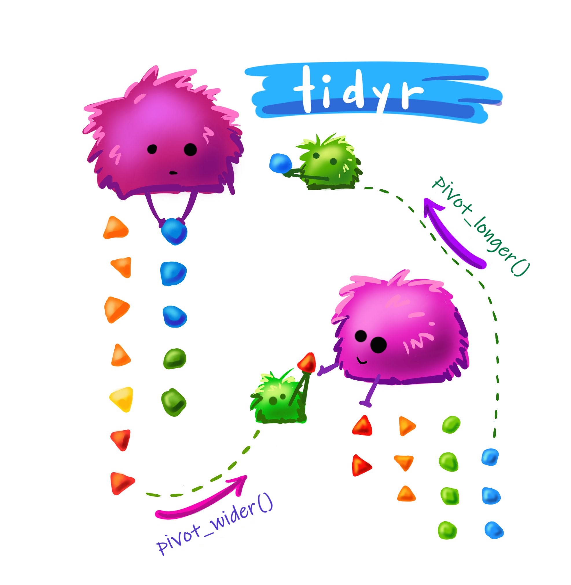
Pivot wider

AE summary steps
Step 1: Summarize participants in population
Step 2: Summarize participants in population by AE criteria of interest
Step 3: Combine summaries
Step 4+: Format using r2rtf
Chapter 8
Section 12.2 Specific AEs
Report each adverse event, the number of patients in each treatment group in whom the event occurred, and the rate of occurrence.
page functions
The AE table introduces us to two advanced table features:
group content: AE can be summarized in multiple nested layers. (e.g., by system organ class (SOC,
AESOC) and specific AE term (AEDECOD))page_by()
pagenization: there are many AE terms that can not be covered in one page. Column headers and SOC information need to be repeated on every page.
pageby_row()
AE tabulation steps
Step 1: Count the number of participants by SOC and treatment arm
Step 2: Count the number of participants in each AE term by SOC, AE term, and treatment arm
Step 3: Count the number of participants in each arm
Step 4: Combine counts
Step 5+: Format the output by using r2rtf
Chapter 9
All TLFs are then assembled by
Combining RTF source code in individual files into one large RTF file.
Leveraging the
Toggle Fieldsfeature in Microsoft Word to embed RTF files using hyperlinks.
Combine source code
Leverage Microsoft Word
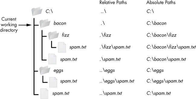
- Absolute paths

- Alt + F9 to “Toggle Fields”